This overview accompanies the IOI Tear Sheet on ArcelorMittal (MT) and is split into the following sections:
- Revenue Scenarios
- Economic Profit Scenarios
- Investment Efficacy Scenarios
- IOI’s explicit forecast period for ArcelorMittal lasts five years.
Revenue Scenarios
We cannot talk about revenue scenarios for ArcelorMittal–the world’s largest steel producer–without talking about the price of steel and of the great commodity supercycle built on emerging market (mainly Chinese) demand.
The first important thing to realize is that the revenues for a commodity producer are going to vary with changes in two factors: volume sold and average selling price. Volumes can remain flat, but if the price goes up by 20%, a commodity producer’s revenues will increase by roughly 20%. If volumes double, but prices drop in half (strange for a steel producer, but not for a producer of NAND flash computer chips…), the revenue of the producer will stay about flat.
So in order to make revenue projections for MT, we looked at both volumes and prices and made some assumptions about best and worst-case scenarios around both.
First for volumes. ArcelorMittal is not terribly exposed to China or India, but instead sells most of its steel into developed Europe, North America, and Brazil. Developed market demand is of course more stable than emerging market demand which limits MT’s growth in a big upturn, but also limits its contraction during a downturn. Here is a chart of historical steel shipments for MT and our best- and worst-case projections.
 |
| ArcelorMittal Steel Shipments (Historical and IOI Projections) Source: Company statements, IOI Analysis |
Note that even in the severe downturn in 2009, MT’s shipments still only decreased by around 25%. In our worst case projections, we take this into account and keep shipments within a few percentage points of what they have been in the past. Our best-case scenario shows shipments increasing gradually with a recovery in developed markets.
The other part of the revenue equation–the price of products sold–requires a bit more explanation. There are many types of steel products sold in this world, all of them with different qualities and different average selling prices (ASPs). ArcelorMittal’s product line is weighted toward more highly-engineered, higher ASP offerings, due in good part because of the quantity of steel they sell into the automotive industry. As such, MT has some control over the prices they charge to clients–their engineering capabilities and scale allow them the ability to charge more for a what many consider a commodity product. That said, the engineered product they sell is, in fact, tied to commodity prices to a greater or lesser extent, so if the price of commodity steel crashes, MT will have to accept a lower price for their offerings.
The following is a chart (courtesy data from IndexMundi.com) of the average price per tonne of four grades of steel (Cold-rolled, Wire rod, Hot-rolled, and Rebar in order of price and value-added) over the past 30 years:
 |
| Average market price of four grades of steel (Source: IndexMundi.com) |
In this chart, the enormous rise in price in the mid-2000s–caused in large part by a rapidly urbanizing China–is clearly visible. (The demarcation of “-30%” will be explained below.)
People in the know term this rise in price (which was, incidentally accompanied with a rise in price of other commodities) as a “commodity supercycle.” Like most terms bandied about in financial circles, it sounds good, but few people understand the particulars. One inference that a lot of people seem to take from the term “supercycle” is that it will last for years and years and will permanently reset “minimum” prices for a given commodity. Certainly, looking at the above chart, one would have a very different opinion about a firm selling steel if one thought that the price would climb yet higher from today or if it would fall back to the prices seen in the late 1990s.
Searching the academic literature to find some hard numbers regarding supercycles, I chanced upon an interesting paper written by two economists on behalf of the United Nations entitled “Super-cycles of commodity prices since the mid-nineteenth century”. I will not go into all the particulars of this paper, but the findings were that there have been four supercycles in metals pricing since the mid-nineteenth century that correspond to various macro-demand events (Railroads, Post-WWII Rebuild, closely followed by the economic ascension of Japan, and China Urbanization). These supercycles tend to be relatively short–lasting from 20-70 years–and are grafted on top of a longer-period trend. A picture is worth a thousand words, so rather than explaining more, I am including a graph included in the above-mentioned paper:
 |
| Source: “Super-cycles of commodity prices since the mid-nineteenth century” DESA Working Paper Series No. 110 by: Bilge Erten and Jose Antonio Ocampo (2012) |
The top-most lines show the real price of steel overlaid by the long-term price trend. The bottom-most lines show the end of the mid-nineteenth century supercycle, followed by the subsequent three. There are good reasons, I believe, to think that the long-term trend will continue to rise into the future, but in terms of the Chinese supercycle, it peaked in 2007 and has been reversing itself in fits and starts since.
Note that after each supercycle, the real trough price drops lower than the previous trough price. As such, there is ample reason to believe that lower steel prices are in the cards as the Chinese urbanization supercycle fades into history.
On the other hand, the longer term trend seems to be upward (again, for what I believe are good economic reasons–namely, technology to remove ore is not not improving much and one of the main inputs to its extraction, oil, is becoming harder and more expensive to mine itself), so the price collapse of steel that would be expected at the end of a supercycle may be ameliorated due to this trend.
As such, to the above shipment numbers, I applied price assumptions of flat (in the best case) to down 30% In the worst case. The 30% line is marked on the chart above–note that a 30% decrease is the high point of pre-supercycle prices. I translated these pricing assumptions into the terms of MT’s historical ASPs to get the following graph:
 |
| Historical and Projected ASPs for MT Source: Company statements, IOI Analysis |
Our worst- and best-case revenue scenarios use the above assumptions for the years 2014-2017 and analyst consensus sales estimates for the present fiscal year. A graph of these projections, compared to historical levels are as follows:
 |
| Historical and Projected Revenues for MT Source: Company Statements, IOI Analysis |
- IOI’s worst case revenue scenario generates an average year-over-year (YoY) nominal growth rate and 5-year compound annual growth rate (5Y CAGR) of -7%.
- IOI’s best case revenue scenario generates an average YoY nominal growth rate of 5% and a 5Y CAGR of 3%.
Economic Profit Scenarios
IOI’s estimate of economic profit deducts an estimate of maintenance capital expenditures from cash flows from operations.
MT management has cut back on all but the most essential capital expenditures for the steel business (which they call maintenance capex), but continues to spend capex dollars on their mining operations (which they term growth capex). IOI’s estimate of maintenance capex is based on depreciation and depreciation expense is much higher than the figure MT publishes for maintenance capex. I continue to use the depreciation-based figure under the assumption that the maintenance numbers the company publishes is the bare-bones expense required to keep the steel operations going through the present downturn. At some point in the future, in order to continue to be a healthy, going concern, MT will have to start spending more to bring its idled steel capacity online and get it in peak operating condition.
Profitability for a steel company is dependent upon the cost of inputs (iron ore, scrap metal, natural gas, etc.). In making our projections, we did not believe that we would necessarily get a more accurate projection of profitability by modeling each and every one of these scenarios. Economic profitability can be controlled to a certain extent by the choices made by company managers (e.g., by idling a plant or bring it back on line depending on business conditions). As such, we modeled MT’s economic profitability by referring to MT’s historical results. This is a perfect example of what theorists call “anchoring bias”, and normally, we would look to avoid this bias, but in this case, we believed it is the best estimate we can give. The lack of precision regarding economic profitability forecasting is one factor prompting us to assign a “Low” conviction rating to the MT valuation. The following graph represents IOI’s estimate of MT’s historical economic profitability and our best- and worst-case projections for the next five years.
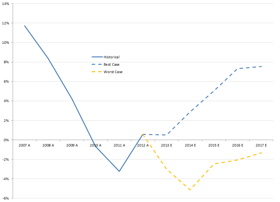 |
| IOI Estimates of MT Economic Profitability Source: Company Statements, IOI Analysis |
- IOI’s worst case profitability scenario generates an average economic profit margin of -3% over the explicit forecast period.
- IOI’s best case profitability scenario generates an average economic profit margin of around 5% over the explicit forecast period.
Investment Efficacy Scenarios
ArcelorMittal is, in essence, an investing company that specializes in steel manufacturers. Lakshmi Mittal’s ability to identify, purchase, and consolidate a diverse portfolio of international steel producers has made him one of the wealthiest people in the world.
That said, any investor operates within a limited timeframe during which secular factors can aid or hinder one’s investing activities. During a paradigm shift, even a very skillful manager can be destroyed by continuing the investment policy he or she followed during a secular upswing.
Mittal has invested a great deal of money in buying mining properties in recent years because the Chinese urbanization supercycle has driven up steel input prices and made them volatile. His investment in mining properties is a form of input cost hedging on a massive scale. Hedging can be thought of as insurance, and we all know from personal experience that much of the money spent on insuring assets is “wasted” through lack of use (of course no one insures their house hoping it will burn down so insurance money can be received). Mittal’s hedging activities may have been wise, or it may have been unnecessary; the answer will only be knowable in a few years and will depend on what happens to steel input costs in the future.
Rather than making a call on this hedging activity, we have made the assumption that a steel company will, over time, grow with the economy at large. As such, we believe scenarios that have worst-case profitability forecasts during the explicit forecast period will likely be coupled with balancing outperformance during the second (implicit) forecast stage and vice versa. Our estimates of real marginal growth of economic profits for MT are as follows:
 |
| IOI Estimate of MT’s Marginal Growth in Economic Profits Source: Company Statements, IOI Analysis |
- IOI’s worst case medium-term (forecast years 6-10) growth scenario implies a growth in nominal free cash flows of 5% per year.
- IOI’s best case medium-term growth scenario implies marginal cash flows 6 percentage points higher than historical GDP growth at roughly 10% per year.